Transformation of signals#
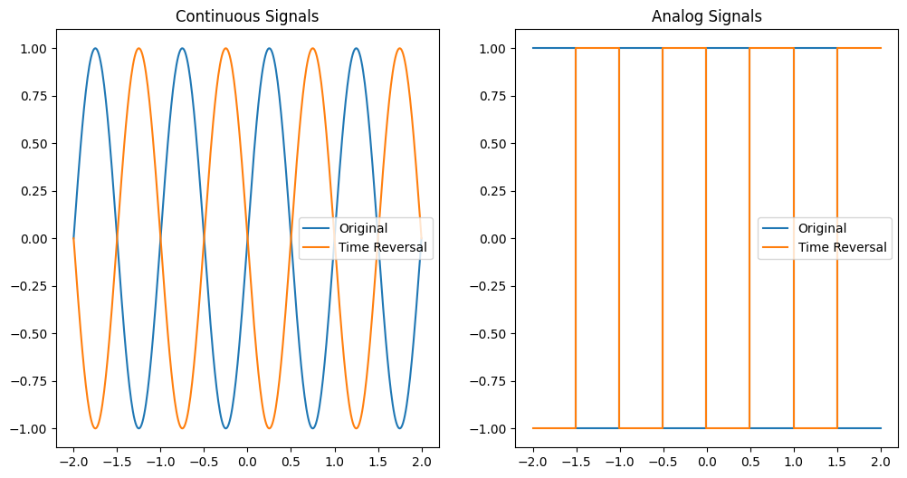
Time Reversal#
Mathematical Equation#
\[ y(t) = x(-t) \]
Explanation#
Time reversal flips the signal around the vertical axis. This means that the signal which occurs at \( t = a \) in the original signal will now occur at \( t = -a \).
import matplotlib.pyplot as plt
import numpy as np

# Define time variable
t = np.linspace(-2, 2, 400)
# Continuous signal (e.g., sine wave)
x = np.sin(2 * np.pi * t)
# Analog signal (e.g., square wave)
analog = np.sign(x)

# Time Reversal
y_time_reversal = x[::-1]
analog_time_reversal = analog[::-1]

# Create subplots
fig, axs = plt.subplots(1, 2, figsize=(12, 6))

# Continuous signals
axs[0].plot(t, x, label='Original')
axs[0].plot(t, y_time_reversal, label='Time Reversal')
axs[0].set_title('Continuous Signals')
axs[0].legend()

# Analog signals
axs[1].plot(t, analog, label='Original', drawstyle='steps-pre')
axs[1].plot(t, analog_time_reversal, label='Time Reversal', drawstyle='steps-pre')
axs[1].set_title('Analog Signals')
axs[1].legend()

plt.show()
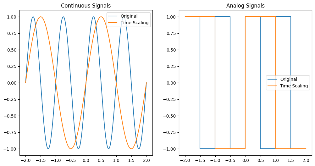
Time Scaling#
Mathematical Equation#
\[ y(t) = x(at) \]
Explanation#
Time scaling compresses or expands the signal. If \( |a| > 1 \), the signal is compressed. If \( |a| < 1 \), the signal is expanded.
a = 0.5
y_time_scaling = np.sin(2 * np.pi * a * t)
analog_time_scaling = np.sign(np.sin(2 * np.pi * a * t))

# Create subplots
fig, axs = plt.subplots(1, 2, figsize=(12, 6))

# Continuous signals
axs[0].plot(t, x, label='Original')
axs[0].plot(t, y_time_scaling, label='Time Scaling')
axs[0].set_title('Continuous Signals')
axs[0].legend()

# Analog signals
axs[1].plot(t, analog, label='Original', drawstyle='steps-pre')
axs[1].plot(t, analog_time_scaling, label='Time Scaling', drawstyle='steps-pre')
axs[1].set_title('Analog Signals')
axs[1].legend()

plt.show()
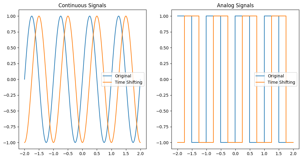
Time Shifting#
Mathematical Equation#
\[ y(t) = x(t - t_0) \]
Explanation#
Time shifting moves the signal along the time axis. If \( t_0 > 0 \), the signal shifts to the right. If \( t_0 < 0 \), the signal shifts to the left.
t0 = 1.25
y_time_shifting = np.sin(2 * np.pi * (t - t0))
analog_time_shifting = np.sign(np.sin(2 * np.pi * (t - t0)))

# Create subplots
fig, axs = plt.subplots(1, 2, figsize=(12, 6))

# Continuous signals
axs[0].plot(t, x, label='Original')
axs[0].plot(t, y_time_shifting, label='Time Shifting')
axs[0].set_title('Continuous Signals')
axs[0].legend()

# Analog signals
axs[1].plot(t, analog, label='Original', drawstyle='steps-pre')
axs[1].plot(t, analog_time_shifting, label='Time Shifting', drawstyle='steps-pre')
axs[1].set_title('Analog Signals')
axs[1].legend()

plt.show()
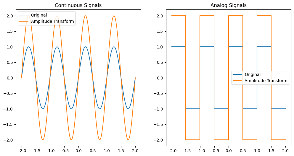
Amplitude Transformation#
Mathematical Equation#
\[ y(t) = a \cdot x(t) \]
Explanation#
Amplitude transformation changes the amplitude of the signal. If \( |a| > 1 \), the signal is amplified. If \( |a| < 1 \), the signal is attenuated.
amp_factor = 2
y_amp_transform = amp_factor * x
analog_amp_transform = amp_factor * analog

# Create subplots
fig, axs = plt.subplots(1, 2, figsize=(12, 6))

# Continuous signals
axs[0].plot(t, x, label='Original')
axs[0].plot(t, y_amp_transform, label='Amplitude Transform')
axs[0].set_title('Continuous Signals')
axs[0].legend()

# Analog signals
axs[1].plot(t, analog, label='Original', drawstyle='steps-pre')
axs[1].plot(t, analog_amp_transform, label='Amplitude Transform', drawstyle='steps-pre')
axs[1].set_title('Analog Signals')
axs[1].legend()

plt.show()
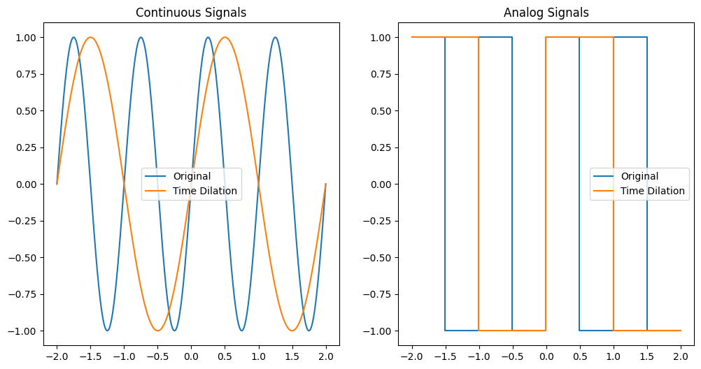
Additional Transformation: Time Dilation#
Mathematical Equation#
\[ y(t) = x(t / a) \]
Explanation#
Time dilation either stretches or compresses the time axis. If \( a > 1 \), the signal is stretched. If \( a < 1 \), the signal is compressed.
dilation_factor = 2
y_time_dilation = np.sin(2 * np.pi * (t / dilation_factor))
analog_time_dilation = np.sign(np.sin(2 * np.pi * (t / dilation_factor)))

# Create subplots
fig, axs = plt.subplots(1, 2, figsize=(12, 6))

# Continuous signals
axs[0].plot(t, x, label='Original')
axs[0].plot(t, y_time_dilation, label='Time Dilation')
axs[0].set_title('Continuous Signals')
axs[0].legend()

# Analog signals
axs[1].plot(t, analog, label='Original', drawstyle='steps-pre')
axs[1].plot(t, analog_time_dilation, label='Time Dilation', drawstyle='steps-pre')
axs[1].set_title('Analog Signals')
axs[1].legend()

plt.show()