Even and Odd Signals

Even Signal Example

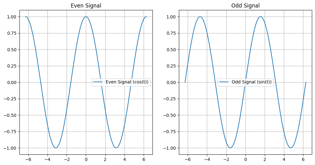
An even signal is symmetric around the vertical axis. A common example of an even signal is the cosine function.

Mathematical Equation

\[ x_{\text{even}}(t) = \cos(t) \]

Explanation

For the cosine function, the property \( \cos(t) = \cos(-t) \) holds true, meaning the signal is identical for positive and negative values of \( t \), making it an even signal.

Odd Signal Example

An odd signal is anti-symmetric around the vertical axis. A common example of an odd signal is the sine function.

Mathematical Equation

\[ x_{\text{odd}}(t) = \sin(t) \]

Explanation

For the sine function, the property \( \sin(t) = -\sin(-t) \) holds true, meaning the signal is the negative of itself for positive and negative values of \( t \), making it an odd signal.

import matplotlib.pyplot as plt
import numpy as np

# Define time variable
t = np.linspace(-2*np.pi, 2*np.pi, 400)
# Even signal (cosine wave)
x_even = np.cos(t)
# Odd signal (sine wave)
x_odd = np.sin(t)

# Create subplots
fig, axs = plt.subplots(1, 2, figsize=(12, 6))

# Even signal plot
axs[0].plot(t, x_even, label='Even Signal (cos(t))')
axs[0].set_title('Even Signal')
axs[0].legend()
axs[0].grid(True)

# Odd signal plot
axs[1].plot(t, x_odd, label='Odd Signal (sin(t))')
axs[1].set_title('Odd Signal')
axs[1].legend()
axs[1].grid(True)

plt.show()

Theory Behind Even and Odd Signals

Even Signal

An even signal \(x(t)\) satisfies the condition:

\[ x(t) = x(-t) \]

This means that the signal is symmetric with respect to the vertical axis. In mathematical terms, for all \(t\), the value of the signal at \(t\) is the same as the value of the signal at \(-t\).

Odd Signal

An odd signal \(x(t)\) satisfies the condition:

\[x(t) = -x(-t)\]

This means that the signal is anti-symmetric with respect to the vertical axis. In mathematical terms, for all \(t\), the value of the signal at \(t\) is the negative of the value of the signal at \(-t\).

By visualizing the even and odd signals, we can see the symmetry and anti-symmetry properties, respectively. This helps in understanding how these signals behave and can be used in signal processing applications.

Signal Summation: Even and Odd Components

Mathematical Equations

For a given signal \( x(t) \), the even and odd components are defined as:

\[ x_{\text{even}}(t) = \frac{1}{2} \left( x(t) + x(-t) \right) \]

\[ x_{\text{odd}}(t) = \frac{1}{2} \left( x(t) - x(-t) \right) \]

Explanation

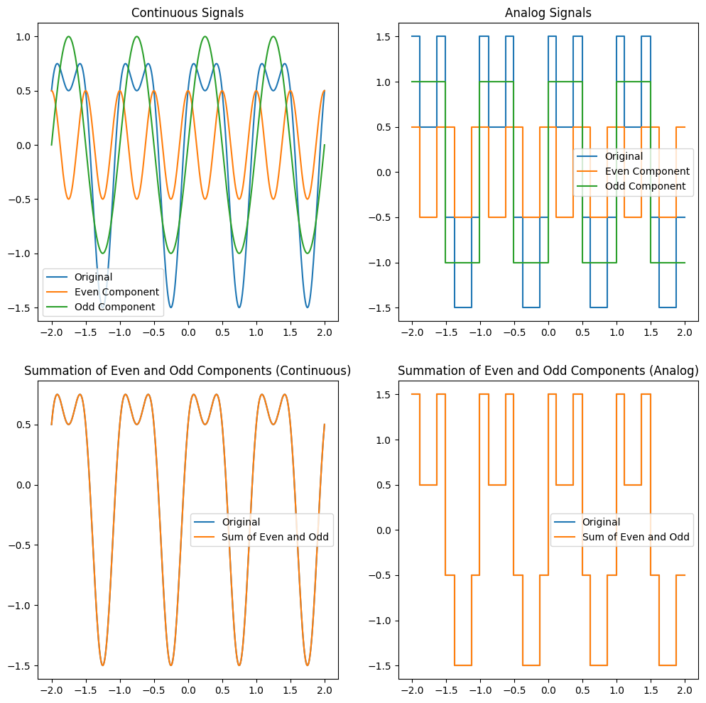
• Even Component: The even component of a signal is symmetric around the vertical axis.

• Odd Component: The odd component of a signal is anti-symmetric around the vertical axis.

import matplotlib.pyplot as plt
import numpy as np

# Define time variable
t = np.linspace(-2, 2, 400)
# Continuous signal (a combination of sine and cosine)
x = np.sin(2 * np.pi * t) + 0.5 * np.cos(4 * np.pi * t)
# Analog signal (a combination of two square waves)
analog = np.sign(np.sin(2 * np.pi * t)) + 0.5 * np.sign(np.cos(4 * np.pi * t))

# Even and Odd Components for Continuous Signal
x_even = 0.5 * (x + x[::-1])
x_odd = 0.5 * (x - x[::-1])

# Even and Odd Components for Analog Signal
analog_even = 0.5 * (analog + analog[::-1])
analog_odd = 0.5 * (analog - analog[::-1])

# Create subplots
fig, axs = plt.subplots(2, 2, figsize=(12, 12))

# Continuous signals
axs[0][0].plot(t, x, label='Original')
axs[0][0].plot(t, x_even, label='Even Component')
axs[0][0].plot(t, x_odd, label='Odd Component')
axs[0][0].set_title('Continuous Signals')
axs[0][0].legend()

# Analog signals
axs[0][1].plot(t, analog, label='Original', drawstyle='steps-pre')
axs[0][1].plot(t, analog_even, label='Even Component', drawstyle='steps-pre')
axs[0][1].plot(t, analog_odd, label='Odd Component', drawstyle='steps-pre')
axs[0][1].set_title('Analog Signals')
axs[0][1].legend()

# Summation of Even and Odd Components for Continuous Signal
x_sum = x_even + x_odd

# Summation of Even and Odd Components for Analog Signal
analog_sum = analog_even + analog_odd

# Continuous signals summation
axs[1][0].plot(t, x, label='Original')
axs[1][0].plot(t, x_sum, label='Sum of Even and Odd')
axs[1][0].set_title('Summation of Even and Odd Components (Continuous)')
axs[1][0].legend()

# Analog signals summation
axs[1][1].plot(t, analog, label='Original', drawstyle='steps-pre')
axs[1][1].plot(t, analog_sum, label='Sum of Even and Odd', drawstyle='steps-pre')
axs[1][1].set_title('Summation of Even and Odd Components (Analog)')
axs[1][1].legend()

plt.show()

This code generates four plots:

1. The original continuous signal with its even and odd components.

2. The original analog signal with its even and odd components.

3. The summation of the even and odd components of the continuous signal compared to the original signal.

4. The summation of the even and odd components of the analog signal compared to the original signal.

By visualizing these plots, we can see how the even and odd components combine to recreate the original signal.