Fourier Transform

The Fourier Transform is a fundamental mathematical tool that enables the transformation of signals and systems from the time domain to the frequency domain. By breaking down a complex signal into its constituent frequencies, it provides insights into the spectral characteristics of the signal, which are crucial for understanding and analyzing various phenomena in fields such as engineering, physics, and signal processing.

Introduction

The Fourier Transform is named after the French mathematician Jean-Baptiste Joseph Fourier, who first formalized the theory in the early 19th century. It serves as a bridge between the time and frequency domains, allowing us to express a time-domain signal as a combination of sinusoids. This transformation is widely applied in signal processing, telecommunications, image processing, and even quantum mechanics to study the frequency behavior of signals and systems.

Theoretical Background and Sufficient Conditions for Existence

The Fourier Transform is defined for a signal \(x(t)\) if the following conditions, known as the Dirichlet conditions, are satisfied:

1. Absolute Integrability: The signal \(x(t)\) must be absolutely integrable over the entire time axis, i.e.,

\[ \int_{-\infty}^{\infty} |x(t)| \, dt < \infty. \]

2. Finite Number of Discontinuities: \(x(t)\) must have a finite number of discontinuities in any given interval.

3. Finite Number of Maxima and Minima: \(x(t)\) must have a finite number of maxima and minima in any given interval.

If these conditions are met, the Fourier Transform exists, and we can use it to represent the signal in the frequency domain. The importance of these conditions lies in ensuring that the resulting frequency representation is both meaningful and mathematically valid.

Definition

Definition 11

The Fourier Transform of a continuous-time signal \(x(t)\) is given by the equation:

\[ \boxed{X(f) = \int_{-\infty}^{\infty} x(t) e^{-j2\pi ft} \, dt} \]

where:

• \(X(f)\) is the frequency domain representation of the signal.

• \(f\) is the frequency variable.

• \(j\) is the imaginary unit (\(j = \sqrt{-1}\)).

• \(e^{-j2\pi ft}\) is the complex exponential function, which serves as the basis function for the transform.

Alternatively, we can express the Fourier Transform using the angular frequency \(\omega\) where \(\omega = 2\pi f\). The transform then becomes:

\[ \boxed{X(\omega) = \int_{-\infty}^{\infty} x(t) e^{-j\omega t} \, dt} \]

The Inverse Fourier Transform allows us to reconstruct the original time-domain signal from its frequency representation:

\[ \boxed{x(t) = \frac{1}{2\pi} \int_{-\infty}^{\infty} X(f) e^{j2\pi ft} \, df} \]

or, equivalently:

\[ \boxed{x(t) = \frac{1}{2\pi} \int_{-\infty}^{\infty} X(\omega) e^{j\omega t} \, d\omega} \]

Interpretation and Application

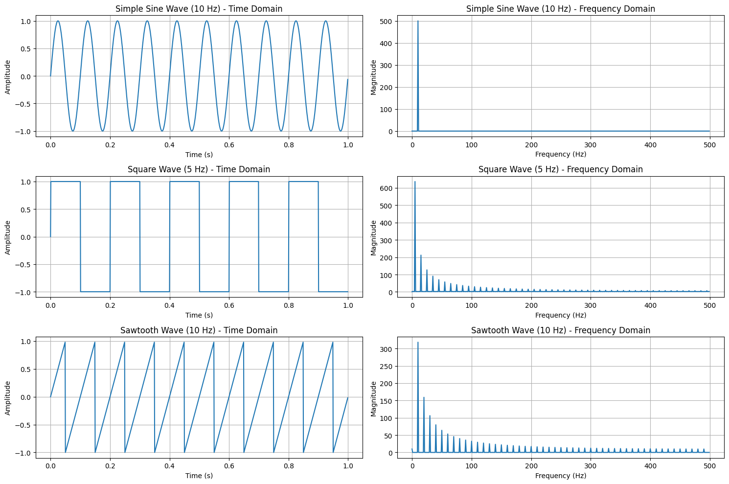
The Fourier Transform essentially decomposes a signal into its sinusoidal components, with each component corresponding to a specific frequency. This decomposition reveals how much of each frequency is present in the original signal, making it invaluable for analyzing periodicity, noise, and system behavior.

In summary, the Fourier Transform is a powerful analytical tool that extends beyond mere mathematical manipulation, offering profound insights into the behavior of signals and systems in the frequency domain.

Let’s see some visual examples of the Fourier Transform

import numpy as np
import matplotlib.pyplot as plt

# Set up the figure and axes
fig, axs = plt.subplots(3, 2, figsize=(15, 10))
plt.subplots_adjust(hspace=0.4, wspace=0.4)

# Time array
t = np.linspace(0, 1, 1000, endpoint=False)

# Function to plot signal and its FFT
def plot_signal_and_fft(t, signal, ax_time, ax_freq, title):
    ax_time.plot(t, signal)
    ax_time.set_xlabel('Time (s)')
    ax_time.set_ylabel('Amplitude')
    ax_time.set_title(f'{title} - Time Domain')
    ax_time.grid(True)

    fft = np.fft.fft(signal)
    freqs = np.fft.fftfreq(len(t), t[1] - t[0])
    ax_freq.plot(freqs[:len(freqs)//2], np.abs(fft)[:len(freqs)//2])
    ax_freq.set_xlabel('Frequency (Hz)')
    ax_freq.set_ylabel('Magnitude')
    ax_freq.set_title(f'{title} - Frequency Domain')
    ax_freq.grid(True)

# 1. Simple sine wave
signal1 = np.sin(2 * np.pi * 10 * t)
plot_signal_and_fft(t, signal1, axs[0, 0], axs[0, 1], "Simple Sine Wave (10 Hz)")

# 2. Square wave
signal2 = np.sign(np.sin(2 * np.pi * 5 * t))
plot_signal_and_fft(t, signal2, axs[1, 0], axs[1, 1], "Square Wave (5 Hz)")

# 3. Sawtooth wave
signal3 = 2 * (t * 10 - np.floor(t * 10 + 0.5))
plot_signal_and_fft(t, signal3, axs[2, 0], axs[2, 1], "Sawtooth Wave (10 Hz)")

# Adjust layout and display
plt.tight_layout()
plt.show()

Impulse Functions in Time Domain

The impulse function, often referred to as the Dirac delta function and denoted by \(\delta(t)\) in the time domain, is a fundamental concept in signal processing and systems theory. It serves as a building block for defining and understanding various signal transformations, including the Fourier Transform. The impulse function is unique in that it is zero everywhere except at \(t = 0\), where it is infinite, yet integrates to 1:

\[ \boxed{\int_{-\infty}^{\infty} \delta(t) \, dt = 1} \]

The Fourier Transform of the impulse function \(\delta(t)\) provides a corresponding impulse-like representation in the frequency domain. This dual nature makes the delta function a key element in the study of signals and their frequency properties.

Mathematical Development

1. Impulse Function in the Time Domain

The Dirac delta function is defined as a limit of a sequence of functions that concentrate all their “area” at a single point, usually \(t = 0\). In the time domain, \(\delta(t)\) is defined by:

\[\begin{split} \delta(t) = \begin{cases} 0, & t \neq 0 \\ \infty, & t = 0 \end{cases} \end{split}\]

with the property:

\[ \int_{-\infty}^{\infty} \delta(t) \, dt = 1 \]

The delta function is primarily used as an idealization of a unit pulse with infinitesimally small width and unit area. For any continuous function \(x(t)\), the sifting property of \(\delta(t)\) is given by:

\[ \int_{-\infty}^{\infty} x(t) \delta(t) \, dt = x(0) \]

2. Impulse Function in the Frequency Domain

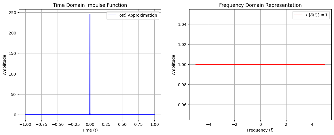
The Fourier Transform of the time-domain impulse function \(\delta(t)\) is a constant function in the frequency domain:

\[ \boxed{ \mathcal{F} \{ \delta(t) \} = \int_{-\infty}^{\infty} \delta(t) e^{-j2\pi ft} \, dt = 1 } \]

This result shows that \(\delta(t)\) contains all frequency components with equal amplitude, which means it has no dominant frequency and is spread uniformly across the spectrum.

3. Inverse Transform

The Inverse Fourier Transform of the frequency-domain constant \(1\) yields back the impulse function in the time domain:

\[ \boxed{ \mathcal{F}^{-1} \{ 1 \} = \int_{-\infty}^{\infty} e^{j2\pi ft} \, df = \delta(t) } \]

This shows that the time-domain impulse \(\delta(t)\) is a unique signal with its frequency domain counterpart being a constant function.

Visualization

To better understand the impulse function and its properties, the following plots illustrate the impulse function in both time and frequency domains. The time-domain plot demonstrates the peak at \(t = 0\), and the frequency-domain plot shows that the transform is a constant across all frequencies.

import numpy as np
import matplotlib.pyplot as plt

# Define the time and frequency range
t = np.linspace(-1, 1, 1000)
f = np.linspace(-5, 5, 1000)

# Time domain impulse approximation using a narrow Gaussian pulse
delta_t = np.exp(-t**2 / (2 * 0.001**2))  # Approximation for delta function
delta_t /= np.trapz(delta_t, t)  # Normalize the area to 1

# Frequency domain is a constant 1 for all frequencies
delta_f = np.ones_like(f)

# Create subplots
fig, (ax1, ax2) = plt.subplots(1, 2, figsize=(14, 5))

# Plot the impulse function in time domain
ax1.plot(t, delta_t, label=r'$\delta(t)$ Approximation', color='b')
ax1.set_title('Time Domain Impulse Function')
ax1.set_xlabel('Time (t)')
ax1.set_ylabel('Amplitude')
ax1.legend()
ax1.grid()

# Plot the impulse function in frequency domain
ax2.plot(f, delta_f, label=r'$\mathcal{F} \{\delta(t)\} = 1$', color='r')
ax2.set_title('Frequency Domain Representation')
ax2.set_xlabel('Frequency (f)')
ax2.set_ylabel('Amplitude')
ax2.legend()
ax2.grid()

# Show plots

/tmp/ipykernel_10267/908283437.py:10: DeprecationWarning: `trapz` is deprecated. Use `trapezoid` instead, or one of the numerical integration functions in `scipy.integrate`.
  delta_t /= np.trapz(delta_t, t)  # Normalize the area to 1

Impulse Functions in the Frequency Domain

Introduction

The impulse function in the frequency domain, denoted by \(\delta(f)\), is a key concept in signal processing. Just as the Dirac delta function \(\delta(t)\) in the time domain represents a signal that is zero everywhere except at \(t = 0\), the frequency-domain delta function \(\delta(f)\) is zero at all frequencies except at \(f = 0\), where it is infinite and has a unit integral. This behavior is mirrored in its Inverse Fourier Transform, resulting in a constant function in the time domain.

Key Property

The frequency-domain impulse \(\delta(f)\) is defined similarly to its time-domain counterpart with the property:

\[ \boxed{ \int_{-\infty}^{\infty} \delta(f) \, df = 1 } \]

This integral property is crucial for maintaining the “unit area” characteristic across the frequency axis. Any signal multiplied by \(\delta(f)\) will have a non-zero value only at \(f = 0\), making it a powerful tool in filtering and signal modulation.

Mathematical Development

1. Impulse Function in the Frequency Domain

The frequency-domain Dirac delta function \(\delta(f)\) is defined by:

\[\begin{split} \delta(f) = \begin{cases} 0, & f \neq 0 \\ \infty, & f = 0 \end{cases} \end{split}\]

with the property:

\[ \int_{-\infty}^{\infty} \delta(f) \, df = 1 \]

This function acts as an idealized unit pulse at the origin in the frequency domain, capturing only the DC (zero-frequency) component.

2. Impulse Function in the Time Domain

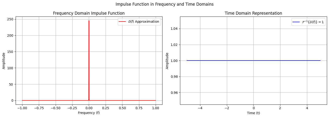
The Inverse Fourier Transform of \(\delta(f)\) gives a constant function in the time domain. This result is mathematically expressed as:

\[ \boxed{ \mathcal{F}^{-1} \{ \delta(f) \} = \int_{-\infty}^{\infty} \delta(f) e^{j2\pi ft} \, df = 1 } \]

This means that the frequency-domain impulse function \(\delta(f)\) corresponds to a constant signal of amplitude 1 at all time values \(t\). In other words, its representation in the time domain is:

\[ \boxed{ \delta(f) \longleftrightarrow 1 \quad \text{in the time domain} } \]

3. Sifting Property in the Frequency Domain

Similar to its counterpart in the time domain, the frequency-domain impulse \(\delta(f)\) has a sifting property when integrated with a function \(X(f)\):

\[ \int_{-\infty}^{\infty} X(f) \delta(f) \, df = X(0) \]

Visualization

The following plots illustrate the impulse function in both frequency and time domains. The frequency-domain plot demonstrates the peak at \(f = 0\), while the time-domain plot shows a constant signal at all time points.

import numpy as np
import matplotlib.pyplot as plt

# Define the time and frequency range
t = np.linspace(-5, 5, 1000)
f = np.linspace(-1, 1, 1000)

# Frequency domain impulse approximation using a narrow Gaussian pulse
delta_f = np.exp(-f**2 / (2 * 0.001**2))  # Approximation for delta function in frequency
delta_f /= np.trapz(delta_f, f)  # Normalize the area to 1

# Time domain is a constant 1 for all time values
delta_t_time = np.ones_like(t)

# Create subplots
fig, (ax1, ax2) = plt.subplots(1, 2, figsize=(14, 5))

# Plot the impulse function in frequency domain
ax1.plot(f, delta_f, label=r'$\delta(f)$ Approximation', color='r')
ax1.set_title('Frequency Domain Impulse Function')
ax1.set_xlabel('Frequency (f)')
ax1.set_ylabel('Amplitude')
ax1.legend()
ax1.grid()

# Plot the constant function in time domain
ax2.plot(t, delta_t_time, label=r'$\mathcal{F}^{-1} \{\delta(f)\} = 1$', color='b')
ax2.set_title('Time Domain Representation')
ax2.set_xlabel('Time (t)')
ax2.set_ylabel('Amplitude')
ax2.legend()
ax2.grid()

# Show plots
plt.suptitle('Impulse Function in Frequency and Time Domains')
plt.tight_layout()
plt.show()

/tmp/ipykernel_10267/3819677020.py:10: DeprecationWarning: `trapz` is deprecated. Use `trapezoid` instead, or one of the numerical integration functions in `scipy.integrate`.
  delta_f /= np.trapz(delta_f, f)  # Normalize the area to 1

Unit Step Function in Time and Frequency Domains

Introduction

The Unit Step Function, denoted as \(u(t)\) in the time domain, is a fundamental building block in signal processing. It is defined to switch from 0 to 1 at a specific point in time, usually at \(t = 0\). This function is widely used to represent signals that “turn on” at a particular instant and remain active indefinitely.

Mathematical Development

1. Definition of the Unit Step Function

The unit step function is defined as:

\[\begin{split} \boxed{u(t) = \begin{cases} 0, & t < 0 \\ 1, & t \geq 0 \end{cases}} \end{split}\]

This function jumps from 0 to 1 at \(t = 0\) and stays constant for \(t \geq 0\). It is primarily used to model signals that switch on and maintain a steady value.

2. Integral Relation with the Impulse Function

The unit step function can be represented as the integral of the impulse function \(\delta(t)\):

\[ \boxed{u(t) = \int_{-\infty}^{t} \delta(\tau) \, d\tau} \]

This relationship shows that \(u(t)\) accumulates the effect of a sudden impulse applied at \(t = 0\), making it a useful tool for analyzing systems’ responses to sudden changes.

3. Fourier Transform of the Unit Step Function

The Fourier Transform of \(u(t)\) is given by:

\[ \boxed{ \mathcal{F} \{ u(t) \} = \frac{1}{j2\pi f} + \frac{1}{2} \delta(f) } \]

This equation states that \(u(t)\) has a decaying imaginary component for non-zero frequencies and a singularity at \(f = 0\). The \(\frac{1}{2} \delta(f)\) term ensures that the Fourier Transform captures the constant behavior of the function for \(t > 0\).

4. Inverse Fourier Transform

The Inverse Fourier Transform of \(U(f)\) results in the original unit step function:

\[ \boxed{ \mathcal{F}^{-1} \left\{ \frac{1}{j2\pi f} + \frac{1}{2} \delta(f) \right\} = u(t) } \]

Interpretation and Application

The unit step function is used to represent signals that suddenly activate and stay on. Its Fourier Transform is useful for understanding the frequency content of such signals, which is dominated by low-frequency components due to the discontinuity at \(t = 0\).

Visualization

The following plots illustrate the unit step function in both the time and frequency domains:

1. Time Domain: The unit step function \(u(t)\) is shown as a sudden jump from 0 to 1.

2. Frequency Domain (Magnitude Response): The magnitude of \(U(f)\) decays as \(\frac{1}{|f|}\) for non-zero frequencies.

3. Frequency Domain (Phase Response): The phase response of \(U(f)\) changes significantly, highlighting the impact of the discontinuity.

import numpy as np
import matplotlib.pyplot as plt

# Define the time range
t = np.linspace(-2, 2, 1000)

# Define the unit step function
u_t = np.heaviside(t, 1)

# Define the frequency range for plotting
f = np.linspace(-10, 10, 1000)

# Frequency response of the unit step function
U_f_mag = np.abs(1 / (1j * 2 * np.pi * f))  # Magnitude response
U_f_phase = np.angle(1 / (1j * 2 * np.pi * f))  # Phase response

# Handle zero value at f = 0 for proper plotting
U_f_mag[500] = 0
U_f_phase[500] = 0

# Create subplots for time and frequency domain representations
fig, (ax1, ax2, ax3) = plt.subplots(1, 3, figsize=(18, 5))

# Plot the unit step function in time domain
ax1.plot(t, u_t, label=r'$u(t)$', color='b')
ax1.set_title('Time Domain: Unit Step Function')
ax1.set_xlabel('Time (t)')
ax1.set_ylabel('Amplitude')
ax1.legend()
ax1.grid()

# Plot the magnitude response in the frequency domain
ax2.plot(f, U_f_mag, label=r'$|U(f)|$', color='r')
ax2.set_title('Frequency Domain: Magnitude Response')
ax2.set_xlabel('Frequency (f)')
ax2.set_ylabel('Magnitude')
ax2.legend()
ax2.grid()

# Plot the phase response in the frequency domain
ax3.plot(f, U_f_phase, label=r'$\angle U(f)$', color='g')
ax3.set_title('Frequency Domain: Phase Response')
ax3.set_xlabel('Frequency (f)')
ax3.set_ylabel('Phase (Radians)')
ax3.legend()
ax3.grid()

# Show plots
plt.suptitle('Unit Step Function: Time and Frequency Domain Representations')
plt.tight_layout()
plt.show()

Exponential Pulse in Time and Frequency Domains

Introduction

The Exponential Pulse is a common signal used in various applications, including filtering, communication systems, and transient analysis. It is characterized by its exponentially decaying nature over time. This pulse is defined for all time \(t\) and is a key example of a non-periodic transient signal. Understanding its time and frequency characteristics provides insight into its application in signal processing and system analysis.

Mathematical Development

1. Definition of the Exponential Pulse

The exponential pulse is defined in the time domain as:

\[ \boxed{x(t) = e^{-\alpha t} u(t)} \]

where:

• \(\alpha > 0\) is the decay constant, which determines how rapidly the signal decays.

• \(u(t)\) is the unit step function ensuring that the pulse exists only for \(t \geq 0\).

• \(e^{-\alpha t}\) represents the exponential decay for \(t \geq 0\).

2. Properties of the Exponential Pulse

1. Decay Rate: The rate of decay is determined by the value of \(\alpha\). A higher value of \(\alpha\) results in a faster decay.

2. Initial Value: At \(t = 0\), \(x(t) = 1\), and as \(t \rightarrow \infty\), \(x(t) \rightarrow 0\).

3. Area Under the Curve: The total energy of the exponential pulse is finite and given by:

\[ \boxed{\int_{0}^{\infty} e^{-\alpha t} \, dt = \frac{1}{\alpha}} \]

This property indicates that the energy of the pulse decreases with an increase in \(\alpha\).

3. Fourier Transform of the Exponential Pulse

The Fourier Transform of \(x(t) = e^{-\alpha t} u(t)\) is given by:

\[ \boxed{ X(f) = \int_{0}^{\infty} e^{-\alpha t} e^{-j2\pi ft} \, dt = \frac{1}{\alpha + j2\pi f} } \]

where \(f\) is the frequency variable. This result shows that the Fourier Transform is a complex function with both magnitude and phase components.

4. Inverse Fourier Transform

The Inverse Fourier Transform of \(X(f)\) results in the original exponential pulse in the time domain:

\[ \boxed{ \mathcal{F}^{-1} \left\{ \frac{1}{\alpha + j2\pi f} \right\} = e^{-\alpha t} u(t) } \]

5. Magnitude and Phase Response

The magnitude and phase of \(X(f)\) are given by:

• Magnitude:

\[ \boxed{ |X(f)| = \frac{1}{\sqrt{\alpha^2 + (2\pi f)^2}} } \]

• Phase:

\[ \boxed{ \angle X(f) = -\tan^{-1} \left( \frac{2\pi f}{\alpha} \right) } \]

6. Visualization

The following plots illustrate the exponential pulse in both time and frequency domains:

1. Time Domain: Shows the exponential decay for \(t \geq 0\).

2. Frequency Domain (Magnitude Response): The magnitude of \(X(f)\) decreases as frequency increases, indicating that higher frequencies have less contribution.

3. Frequency Domain (Phase Response): The phase response varies with frequency, reflecting the frequency-dependent nature of the signal.

import numpy as np
import matplotlib.pyplot as plt

# Parameters for the exponential pulse
alpha = 1  # Decay constant

# Define the time range
t = np.linspace(-1, 5, 1000)

# Define the exponential pulse function
x_t = np.exp(-alpha * t) * (t >= 0)  # Exponential decay for t >= 0

# Define the frequency range for plotting
f = np.linspace(-10, 10, 1000)

# Frequency response of the exponential pulse
X_f = 1 / (alpha + 1j * 2 * np.pi * f)  # Fourier Transform of e^(-alpha*t)u(t)

# Calculate magnitude and phase
X_f_mag = np.abs(X_f)  # Magnitude response
X_f_phase = np.angle(X_f)  # Phase response

# Create subplots for time and frequency domain representations
fig, (ax1, ax2, ax3) = plt.subplots(1, 3, figsize=(18, 5))

# Plot the exponential pulse in time domain
ax1.plot(t, x_t, label=r'$e^{-\alpha t} u(t)$', color='b')
ax1.set_title('Time Domain: Exponential Pulse')
ax1.set_xlabel('Time (t)')
ax1.set_ylabel('Amplitude')
ax1.legend()
ax1.grid()

# Plot the magnitude response in the frequency domain
ax2.plot(f, X_f_mag, label=r'$|X(f)|$', color='r')
ax2.set_title('Frequency Domain: Magnitude Response')
ax2.set_xlabel('Frequency (f)')
ax2.set_ylabel('Magnitude')
ax2.legend()
ax2.grid()

# Plot the phase response in the frequency domain
ax3.plot(f, X_f_phase, label=r'$\angle X(f)$', color='g')
ax3.set_title('Frequency Domain: Phase Response')
ax3.set_xlabel('Frequency (f)')
ax3.set_ylabel('Phase (Radians)')
ax3.legend()
ax3.grid()

# Show plots
plt.suptitle('Exponential Pulse: Time and Frequency Domain Representations')
plt.tight_layout()
plt.show()