Common Signals in Engineering

Continous Signals

A signal that appears often in models is one whose time rate of change is directly proportional to the signal itself.

An example of this type of signal is the differential equation:

\[\frac{dx(t)}{dt} = a x(t)\]

The solution of this equation is the exponential function:

\[x(t) = x(0)e^{at}, \text{ for } t \geq 0\]

The circuit shown below, known as the RL circuit, presents this kind of equation.

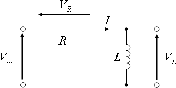
Fig. 1 RL circuit schematic

That is,

\[L\frac{di(t)}{dt} + Ri(t) = 0 \implies \frac{di(t)}{dt} = -\frac{R}{L} i(t) = a i(t), \text{ where } a = -\frac{R}{L}\]

The current is then:

\[i(t) = i(0) e^{-\frac{Rt}{L}}\]

With that in mind, since such signals are common in engineering, let’s proceed with a more general form of such a signal.

\[ x(t) = Ce^{at} \]

where \( C \) and \( a \) can be real or complex number.

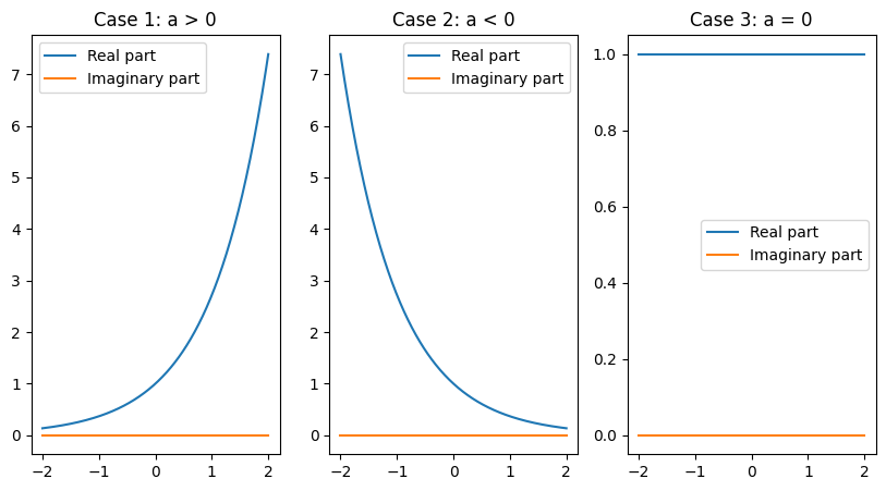
Case 1: \( C \) and \( a \) are Real

\[ x(t) = Ce^{at} \]

This represents an exponential growth or decay depending on the sign of \( a \).

import matplotlib.pyplot as plt
import numpy as np

# Define time variable
t = np.linspace(-2, 2, 400)

# Case 1: a > 0
C1 = 1
a1 = 1
x1 = C1 * np.exp(a1 * t)

# Case 2: a < 0
C2 = 1
a2 = -1
x2 = C2 * np.exp(a2 * t)

# Case 3: a = 0
C3 = 1
a3 = 0
x3 = C3 * np.exp(a3 * t)

# Create subplots
fig, axs = plt.subplots(1, 3, figsize=(10, 5))

# Case 1: a > 0
axs[0].plot(t, x1.real, label='Real part')
axs[0].plot(t, x1.imag, label='Imaginary part')
axs[0].set_title('Case 1: a > 0')
axs[0].legend()

# Case 2: a < 0
axs[1].plot(t, x2.real, label='Real part')
axs[1].plot(t, x2.imag, label='Imaginary part')
axs[1].set_title('Case 2: a < 0')
axs[1].legend()

# Case 3: a = 0
axs[2].plot(t, x3.real, label='Real part')
axs[2].plot(t, x3.imag, label='Imaginary part')
axs[2].set_title('Case 3: a = 0')
axs[2].legend()

plt.show()

To aid us in differentiating between exponentials that decay at different rates, we express the exponential as, for \(a < 0\),

\[x(t) = Ce^{at} = Ce^{\frac{-t}{\tau}}, \quad \tau > 0\]

where \(\tau\) is a time constant of the exponential.

The derivative of \(x(t)\) at \(t = 0\) is given by

\[\frac{dx(t)}{dt}\bigg|_{t=0} = -\frac{C}{\tau}e^{\frac{-t}{\tau}}\bigg|_{t = 0} = -\frac{C}{\tau}\]

import numpy as np
import matplotlib.pyplot as plt

# Parameters
C = 1
a = -1
tau = -1 / a

# Time array
t = np.linspace(0, 5 * tau, 400)

# Exponential function
x_t = C * np.exp(a * t)

# Value of x(t) at t = tau
x_tau = C * np.exp(a * tau)

# Plotting
plt.figure(figsize=(10, 6))
plt.plot(t, x_t, label='$x(t) = Ce^{at} = Ce^{\\frac{-t}{\\tau}}$')
plt.axvline(x=tau, color='r', linestyle='--', label='$t = \\tau$')
plt.scatter([tau], [x_tau], color='r')  # Point at t = tau

# Annotating the point
plt.annotate(f'$x(\\tau) = {x_tau:.3f}$', xy=(tau, x_tau), xytext=(tau + tau * 0.5, x_tau * 0.8),
             arrowprops=dict(facecolor='black', shrink=0.05))

# Adding labels and title
plt.xlabel('Time $t$')
plt.ylabel('$x(t)$')
plt.title('Exponential Decay Function')
plt.legend()
plt.grid(True)
plt.show()

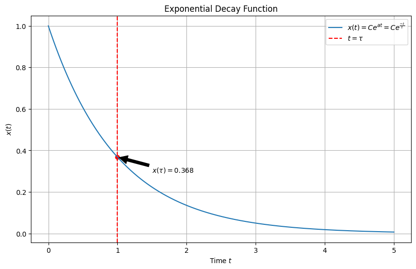
→ Note that the value of the signal at \(t = \tau\) is equal to \(0.368C\); that is, the signal has decayed to \(36.8\%\) of its amplitude after \(\tau\) seconds

Case 2: \(C\) is Complex, \(a\) is Imaginary

\[x(t) = Ce^{at}; \quad C = Ae^{j \phi} = A \angle \phi, \quad a = j\omega_0\]

where \(C\) is complex, \(j\) is the imaginary unit, and \(\omega_0, A, \phi\) are real numbers. This represents a sinusoidal signal with an exponential amplitude modulation.

import matplotlib.pyplot as plt
import numpy as np

# Define time variable
t = np.linspace(-2, 2, 400)

# Case 1: C and a real
C1 = 1
a1 = 1
x1 = C1 * np.exp(a1 * t)

# Case 2: C complex, a imaginary
C2 = 1 + 1j
omega = np.pi
x2 = np.abs(C2) * np.exp(1j * omega * t)

# Create subplots
fig, plt = plt.subplots(figsize=(15, 7))

# Case 1: C and a real
plt.plot(t, x2.real, label='Real part')
plt.plot(t, x2.imag, label='Imaginary part')
plt.set_title('Case 2: C Complex, a Imaginary')
plt.legend();

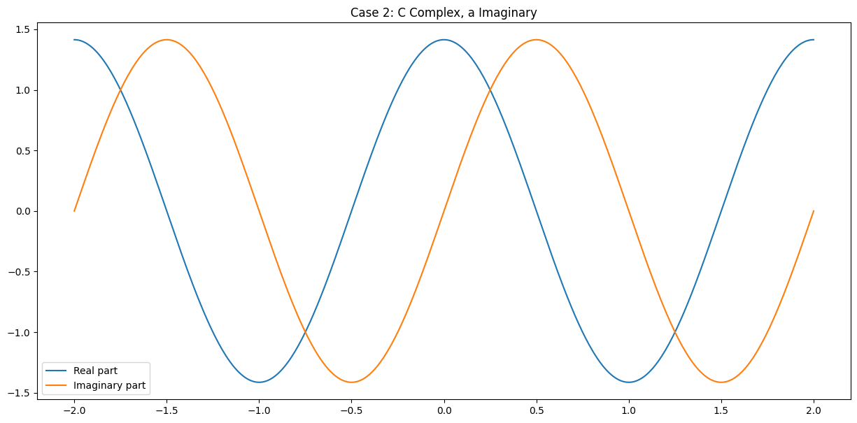
→ Harmonocally related complex exponentials are a set of functions with frequencies related by integers of the form \(x_k(t) = A_k e^{jk \omega_0 t}, k = \pm 1, \pm 2, \cdots\)

Case 3: Both \(C\) and \(a\) are Complex

\[x(t) = Ce^{at}; \quad C = Ae^{j \phi} = A \angle \phi, \quad a = \sigma_0 + j\omega_0\]

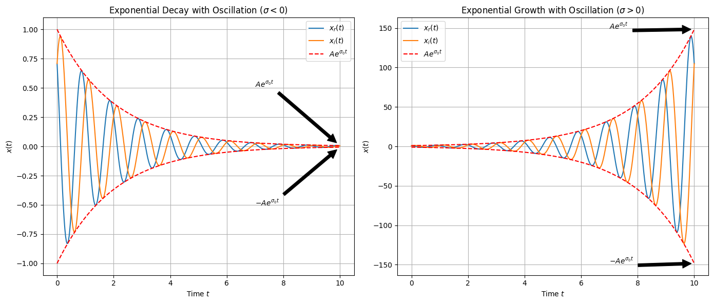
where \(A\), \(\phi\), \(\sigma_0\), and \(\omega_0\) are real and constant. This represents a signal that has both exponential growth/decay and oscillatory behavior. We can represent this signal as,

\[x(t) = Ae^{j \phi}e^{(\sigma_0 + j\omega_0)t} = Ae^{\sigma_0 t}e^{j(\omega_0 t + \phi)}\]

\[x(t) = Ae^{\sigma_0 t}\cos(\omega_0 t + \phi) + jAe^{\sigma_0 t}\sin(\omega_0 t + \phi)\]

\[x(t) = x_r(t) + jx_i(t)\]

where \(r\) stands for real and \(i\) stands for imaginary.

import numpy as np
import matplotlib.pyplot as plt

# Parameters
A = 1
phi = np.pi / 4
omega_0 = 2 * np.pi
sigma_neg = -0.5
sigma_pos = 0.5

# Time array
t = np.linspace(0, 10, 400)

# Exponential decay with oscillation (sigma < 0)
x_decay = A * np.exp((sigma_neg + 1j * omega_0) * t)
x_decay_real = np.real(x_decay * np.exp(1j * phi))
x_decay_imag = np.imag(x_decay * np.exp(1j * phi))
envelope_decay = A * np.exp(sigma_neg * t)

# Exponential growth with oscillation (sigma > 0)
x_growth = A * np.exp((sigma_pos + 1j * omega_0) * t)
x_growth_real = np.real(x_growth * np.exp(1j * phi))
x_growth_imag = np.imag(x_growth * np.exp(1j * phi))
envelope_growth = A * np.exp(sigma_pos * t)

# Plotting
fig, axs = plt.subplots(1, 2, figsize=(14, 6))

# Plot for sigma < 0
axs[0].plot(t, x_decay_real, label='$x_r(t)$')
axs[0].plot(t, x_decay_imag, label='$x_i(t)$')
axs[0].plot(t, envelope_decay, 'r--', label='$Ae^{\sigma_0 t}$')
axs[0].plot(t, -envelope_decay, 'r--')
axs[0].annotate('$Ae^{\sigma_0 t}$', xy=(t[-1], envelope_decay[-1]), xytext=(t[-1] - 3, envelope_decay[-1] + 0.5),
                arrowprops=dict(facecolor='black', shrink=0.05))
axs[0].annotate('$-Ae^{\sigma_0 t}$', xy=(t[-1], -envelope_decay[-1]), xytext=(t[-1] - 3, -envelope_decay[-1] - 0.5),
                arrowprops=dict(facecolor='black', shrink=0.05))
axs[0].set_title('Exponential Decay with Oscillation ($\sigma < 0$)')
axs[0].set_xlabel('Time $t$')
axs[0].set_ylabel('$x(t)$')
axs[0].legend()
axs[0].grid(True)

# Plot for sigma > 0
axs[1].plot(t, x_growth_real, label='$x_r(t)$')
axs[1].plot(t, x_growth_imag, label='$x_i(t)$')
axs[1].plot(t, envelope_growth, 'r--', label='$Ae^{\sigma_0 t}$')
axs[1].plot(t, -envelope_growth, 'r--')
axs[1].annotate('$Ae^{\sigma_0 t}$', xy=(t[-1], envelope_growth[-1]), xytext=(t[-1] - 3, envelope_growth[-1] + 0.5),
                arrowprops=dict(facecolor='black', shrink=0.05))
axs[1].annotate('$-Ae^{\sigma_0 t}$', xy=(t[-1], -envelope_growth[-1]), xytext=(t[-1] - 3, -envelope_growth[-1] - 0.5),
                arrowprops=dict(facecolor='black', shrink=0.05))
axs[1].set_title('Exponential Growth with Oscillation ($\sigma > 0$)')
axs[1].set_xlabel('Time $t$')
axs[1].set_ylabel('$x(t)$')
axs[1].legend()
axs[1].grid(True)

plt.tight_layout()
plt.show()

<>:32: SyntaxWarning: invalid escape sequence '\s'
<>:34: SyntaxWarning: invalid escape sequence '\s'
<>:36: SyntaxWarning: invalid escape sequence '\s'
<>:38: SyntaxWarning: invalid escape sequence '\s'
<>:47: SyntaxWarning: invalid escape sequence '\s'
<>:49: SyntaxWarning: invalid escape sequence '\s'
<>:51: SyntaxWarning: invalid escape sequence '\s'
<>:53: SyntaxWarning: invalid escape sequence '\s'
<>:32: SyntaxWarning: invalid escape sequence '\s'
<>:34: SyntaxWarning: invalid escape sequence '\s'
<>:36: SyntaxWarning: invalid escape sequence '\s'
<>:38: SyntaxWarning: invalid escape sequence '\s'
<>:47: SyntaxWarning: invalid escape sequence '\s'
<>:49: SyntaxWarning: invalid escape sequence '\s'
<>:51: SyntaxWarning: invalid escape sequence '\s'
<>:53: SyntaxWarning: invalid escape sequence '\s'
/tmp/ipykernel_10167/3810044617.py:32: SyntaxWarning: invalid escape sequence '\s'
  axs[0].plot(t, envelope_decay, 'r--', label='$Ae^{\sigma_0 t}$')
/tmp/ipykernel_10167/3810044617.py:34: SyntaxWarning: invalid escape sequence '\s'
  axs[0].annotate('$Ae^{\sigma_0 t}$', xy=(t[-1], envelope_decay[-1]), xytext=(t[-1] - 3, envelope_decay[-1] + 0.5),
/tmp/ipykernel_10167/3810044617.py:36: SyntaxWarning: invalid escape sequence '\s'
  axs[0].annotate('$-Ae^{\sigma_0 t}$', xy=(t[-1], -envelope_decay[-1]), xytext=(t[-1] - 3, -envelope_decay[-1] - 0.5),
/tmp/ipykernel_10167/3810044617.py:38: SyntaxWarning: invalid escape sequence '\s'
  axs[0].set_title('Exponential Decay with Oscillation ($\sigma < 0$)')
/tmp/ipykernel_10167/3810044617.py:47: SyntaxWarning: invalid escape sequence '\s'
  axs[1].plot(t, envelope_growth, 'r--', label='$Ae^{\sigma_0 t}$')
/tmp/ipykernel_10167/3810044617.py:49: SyntaxWarning: invalid escape sequence '\s'
  axs[1].annotate('$Ae^{\sigma_0 t}$', xy=(t[-1], envelope_growth[-1]), xytext=(t[-1] - 3, envelope_growth[-1] + 0.5),
/tmp/ipykernel_10167/3810044617.py:51: SyntaxWarning: invalid escape sequence '\s'
  axs[1].annotate('$-Ae^{\sigma_0 t}$', xy=(t[-1], -envelope_growth[-1]), xytext=(t[-1] - 3, -envelope_growth[-1] - 0.5),
/tmp/ipykernel_10167/3810044617.py:53: SyntaxWarning: invalid escape sequence '\s'
  axs[1].set_title('Exponential Growth with Oscillation ($\sigma > 0$)')

Euler’s Relation

This is a relation that is often applied, which is named Euler’s relation, given by

\[e^{j\theta} = \cos(\theta) + j\sin(\theta)\]

and

\[\cos(\theta) = \frac{e^{j\theta} + e^{-j\theta}}{2}\]

\[\sin(\theta) = \frac{e^{j\theta} - e^{-j\theta}}{2j}\]

Summary

1. Case 1: \( C \) and \( a \) Real (Undamped)

   • This scenario illustrates exponential growth or decay depending on the sign of \( a \). If \( a \) is positive, the signal grows exponentially. If \( a \) is negative, the signal decays exponentially.

2. Case 2: \( C \) Complex, \( a \) Imaginary (Underdamped)

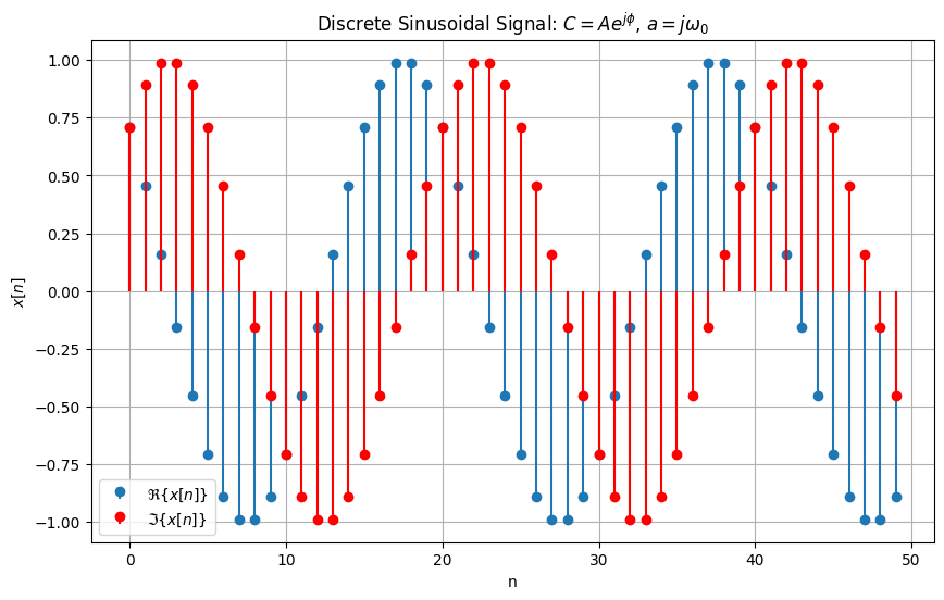
   • This scenario represents a sinusoidal signal with exponential amplitude modulation. The signal oscillates sinusoidally, and the real and imaginary parts both exhibit this oscillatory behavior.

3. Case 3: Both \( C \) and \( a \) Complex (Critically Damped)

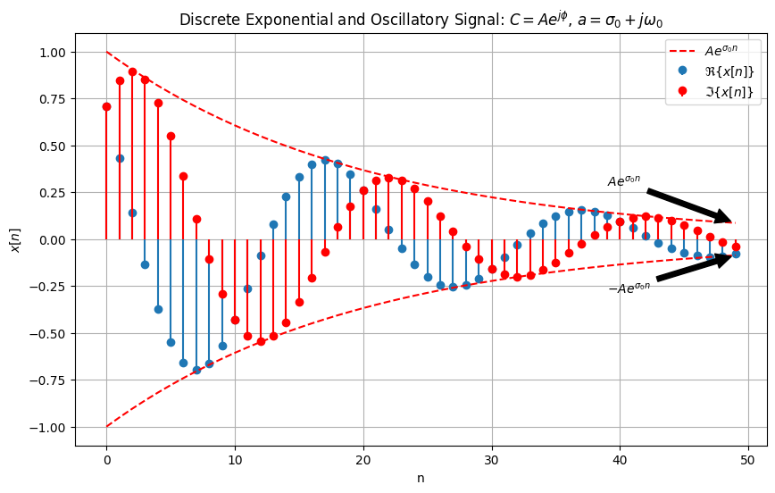
   • This scenario combines exponential growth/decay with oscillatory behavior. The signal exhibits both exponential and sinusoidal characteristics in its real and imaginary parts.

By visualizing these cases, you can observe how different values of \( C \) and \( a \) influence the signal’s behavior.

Discrete Signals

When working with discrete signals, we often encounter scenarios similar to those in continuous-time signals but in a discrete context. Let’s explore the behavior of discrete-time signals through several cases. We’ll use Python code examples to illustrate these concepts.

Discrete-Time Signal Generation

Let’s see again an example of discrete-time signal generation. Imagine we use a computer to output a discrete-time sinusoid to generate an audible tone of variable frequency. For this, we need some element able to store a number. Devices such as registers or memory locations can do this for us. Consider a system where we have an ideal time delay (ITD) which receives an input \( x[n] \) and outputs \( x[n-1] \). Every \( T \) seconds, we shift out the number stored in the device, then a different number is shifted into the device and stored. Next, we connect our delay with a multiplication constant \( a \) such that

\[ x[n] = ax[n - 1] \]

Let’s solve this equation for some outputs:

\[ x[1] = ax[0] = a \]

\[ x[2] = ax[1] = a^2 \]

\[ x[3] = ax[2] = a^3 \]

\[ \vdots \]

\[ x[n] = a^n \]

The system generates the signal \( x[n] = a^n \) for the initial condition \( x[0] = 1 \).

Characteristics of Discrete Signals

Let’s investigate the characteristics of the discrete signal \( x[n] = a^n \). If we let \( a = e^b \), we can express this signal as a discrete-time exponential function. Then,

\[ x[n] = a^n = (e^b)^n = e^{bn} \]

which implies \( x[n] = (e^{\frac{-T}{\tau}})^n = a^n \),

where \( \frac{T}{\tau} \) is the number of samples per time constant. Therefore,

\[ \tau = \frac{-T}{\ln(a)} \]

For example, if \( x[n] = 0.9^n \), then \( 0.9 = e^b \) implies \( b = \ln(0.9) = -0.105 \).

For \( x[n] = 0.8^n \):

\[ \tau = \frac{T}{\ln(a)} \implies \frac{\tau}{T} = -\frac{1}{\ln(0.8)} \implies \tau = 4.48T \]

This means there are 4.478 samples per time constant. Assuming that an exponential decays to a negligible amplitude after four time constants, the signal can be ignored for \( nT > 4\tau \approx 18T \), i.e., \( n > 18 \) samples.

Case 1: \( C \) and \( a \) are Real

For \( C \) and \( a \) real, the discrete signal can be represented as:

\[ x[n] = Ce^{an} \]

This represents an exponential growth or decay depending on the sign of \( a \).

import numpy as np
import matplotlib.pyplot as plt

# Case 1: Discrete exponential signals for different values of 'a'

# Define discrete time variable
n = np.arange(0, 50)

# Case 1: a > 0
C1 = 1
a1 = 0.1
x1 = C1 * np.exp(a1 * n)

# Case 2: a < 0
C2 = 1
a2 = -0.1
x2 = C2 * np.exp(a2 * n)

# Case 3: a = 0
C3 = 1
a3 = 0
x3 = C3 * np.exp(a3 * n)

# Create subplots
fig, axs = plt.subplots(1, 3, figsize=(18, 6))

# Case 1: a > 0
axs[0].stem(n, x1, basefmt=" ")
axs[0].set_title('Case 1: $a > 0$')
axs[0].set_xlabel('n')
axs[0].set_ylabel('$x[n]$')
axs[0].grid(True)

# Case 2: a < 0
axs[1].stem(n, x2, basefmt=" ")
axs[1].set_title('Case 2: $a < 0$')
axs[1].set_xlabel('n')
axs[1].set_ylabel('$x[n]$')
axs[1].grid(True)

# Case 3: a = 0
axs[2].stem(n, x3, basefmt=" ")
axs[2].set_title('Case 3: $a = 0$')
axs[2].set_xlabel('n')
axs[2].set_ylabel('$x[n]$')
axs[2].grid(True)

plt.tight_layout()
plt.show()

Case 2: \( C \) is Complex, \( a \) is Imaginary

For \( C \) complex and \( a \) imaginary:

\[ x[n] = Ce^{an}; \quad C = Ae^{j \phi} = A \angle \phi, \quad a = j\omega_0 \]

where \( C \) is complex, \( j \) is the imaginary unit, and \( \omega_0 \), \( A \), \( \phi \) are real numbers. This represents a sinusoidal signal with an exponential amplitude modulation.

import numpy as np
import matplotlib.pyplot as plt

# Parameters
A = 1
phi = np.pi / 4
omega_0 = 0.1 * np.pi
n = np.arange(0, 50)
x_n = A * np.exp(1j * (omega_0 * n + phi))

# Plotting
plt.figure(figsize=(10, 6))
plt.stem(n, np.real(x_n), label='$\\Re\\{x[n]\\}$', basefmt=" ")
plt.stem(n, np.imag(x_n), label='$\\Im\\{x[n]\\}$', basefmt=" ", linefmt='r', markerfmt='ro')
plt.title('Discrete Sinusoidal Signal: $C = Ae^{j \\phi}$, $a = j\\omega_0$')
plt.xlabel('n')
plt.ylabel('$x[n]$')
plt.legend()
plt.grid(True)
plt.show()

Case 3: Both \( C \) and \( a \) are Complex

For both \( C \) and \( a \) complex:

\[ x[n] = Ce^{an}; \quad C = Ae^{j \phi} = A \angle \phi, \quad a = \sigma_0 + j\omega_0 \]

where \( A \), \( \phi \), \( \sigma_0 \), and \( \omega_0 \) are real and constant. This represents a signal that has both exponential growth/decay and oscillatory behavior. We can represent this signal as:

\[ x[n] = Ae^{j \phi}e^{(\sigma_0 + j\omega_0)n} = Ae^{\sigma_0 n}e^{j(\omega_0 n + \phi)} \]

\[ x[n] = Ae^{\sigma_0 n}\cos(\omega_0 n + \phi) + jAe^{\sigma_0 n}\sin(\omega_0 n + \phi) \]

\[ x[n] = x_r[n] + jx_i[n] \]

where \( r \) stands for real and \( i \) stands for imaginary.

import numpy as np
import matplotlib.pyplot as plt

# Parameters
A = 1
phi = np.pi / 4
sigma_0 = -0.05  # Decay
omega_0 = 0.1 * np.pi
n = np.arange(0, 50)
x_n = A * np.exp((sigma_0 + 1j * omega_0) * n + 1j * phi)

# Envelope functions
envelope = A * np.exp(sigma_0 * n)

# Plotting
plt.figure(figsize=(10, 6))
plt.stem(n, np.real(x_n), label='$\\Re\\{x[n]\\}$', basefmt=" ")
plt.stem(n, np.imag(x_n), label='$\\Im\\{x[n]\\}$', basefmt=" ", linefmt='r', markerfmt='ro')
plt.plot(n, envelope, 'r--', label='$Ae^{\\sigma_0 n}$')
plt.plot(n, -envelope, 'r--')
plt.annotate('$Ae^{\\sigma_0 n}$', xy=(n[-1], envelope[-1]), xytext=(n[-1] - 10, envelope[-1] + 0.2),
             arrowprops=dict(facecolor='black', shrink=0.05))
plt.annotate('$-Ae^{\\sigma_0 n}$', xy=(n[-1], -envelope[-1]), xytext=(n[-1] - 10, -envelope[-1] - 0.2),
             arrowprops=dict(facecolor='black', shrink=0.05))
plt.title('Discrete Exponential and Oscillatory Signal: $C = Ae^{j \\phi}$, $a = \\sigma_0 + j\\omega_0$')
plt.xlabel('n')
plt.ylabel('$x[n]$')
plt.legend()
plt.grid(True)
plt.show()

Summary Table

Case	Equation	Description
\( C \) and \( a \) Real	\( x[n] = Ce^{an} \)	Exponential growth/decay
\( C \) Complex, \( a \) Imaginary	\( x[n] = Ce^{an}; \quad C = Ae^{j \phi}, \quad a = j\omega_0 \)	Sinusoidal signal with exponential amplitude modulation
Both \( C \) and \( a \) Complex	\( x[n] = Ce^{an}; \quad C = Ae^{j \phi}, \quad a = \sigma_0 + j\omega_0 \)	Exponential growth/decay with oscillatory behavior

These examples and explanations illustrate the different types of discrete signals and their characteristics. The Python code provides visualizations to help understand these concepts better.