Fourier Transform Pairs and Its Applications#
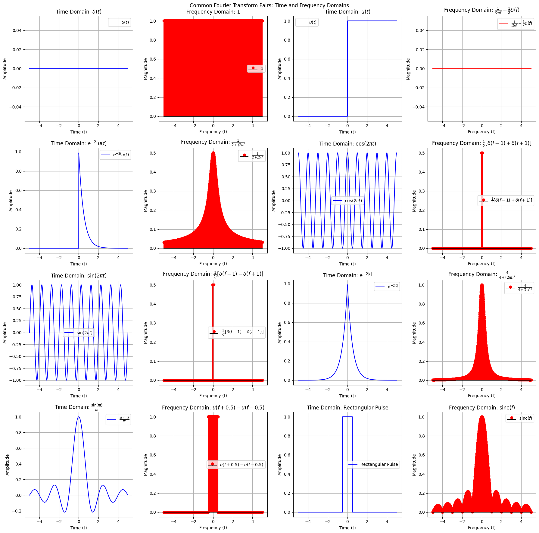
This table summarizes some of the most commonly encountered Fourier Transform pairs, showing the time-domain functions and their corresponding frequency-domain representations. For a complete reference please refer to the following link: https://ethz.ch/content/dam/ethz/special-interest/baug/ibk/structural-mechanics-dam/education/identmeth/fourier.pdf
Time Domain |
Frequency Domain |
|---|---|
\( \delta(t) \) |
\( 1 \) |
\( 1 \) |
\( \delta(f) \) |
\( u(t) \) |
\( \frac{1}{j2\pi f} + \frac{1}{2} \delta(f) \) |
\( e^{- \alpha t} u(t) \) |
\( \frac{1}{\alpha + j2\pi f} \) |
\( e^{j2\pi f_0 t} \) |
\( \delta(f - f_0) \) |
\( \cos(2\pi f_0 t) \) |
\( \frac{1}{2} [ \delta(f - f_0) + \delta(f + f_0) ] \) |
\( \sin(2\pi f_0 t) \) |
\( \frac{1}{2j} [ \delta(f - f_0) - \delta(f + f_0) ] \) |
$ e^{-a |
t |
\( \frac{\sin(\pi f_0 t)}{\pi t} \) |
\( u\left( f + \frac{f_0}{2} \right) - u\left( f - \frac{f_0}{2} \right) \) |
Let’s visualize some Fourier Transform pairs:
import numpy as np
import matplotlib.pyplot as plt

# Define a range for time and frequency
t = np.linspace(-5, 5, 1000)
f = np.linspace(-5, 5, 1000)

# Define common time-domain functions
delta_t = np.zeros_like(t)
delta_t[np.abs(t) < 0.005] = 1  # Approximation for delta function

u_t = np.heaviside(t, 1)  # Unit step function
exp_pulse = np.exp(-2 * t) * (t >= 0)  # Exponential pulse
cos_t = np.cos(2 * np.pi * t)  # Cosine function
sin_t = np.sin(2 * np.pi * t)  # Sine function
exp_abs_t = np.exp(-2 * np.abs(t))  # Exponential decay for all t
sinc_t = np.sinc(t)  # Sinc function
rect_t = np.heaviside(t + 0.5, 1) - np.heaviside(t - 0.5, 1)  # Rectangular pulse

# Fourier Transform pairs' frequency responses
delta_f = np.ones_like(f)  # Fourier Transform of delta(t) is 1
u_f = 1 / (1j * 2 * np.pi * f) + 0.5 * delta_t  # Fourier Transform of u(t)
exp_pulse_f = 1 / (2 + 1j * 2 * np.pi * f)  # Fourier Transform of exp(-2t)u(t)
cos_f = np.zeros_like(f)
cos_f[495] = 0.5  # Positive frequency impulse for cosine at f = 1
cos_f[505] = 0.5  # Negative frequency impulse for cosine at f = -1

# Handling sine function separately using magnitude for vertical lines
sin_f = np.zeros_like(f)
sin_f[495] = 0.5  # Positive frequency impulse for sine at f = 1
sin_f[505] = 0.5  # Negative frequency impulse for sine at f = -1

exp_abs_f = 4 / (4 + (2 * np.pi * f) ** 2)  # Fourier Transform of exp(-2|t|)
sinc_f = np.heaviside(f + 0.5, 1) - np.heaviside(f - 0.5, 1)  # Sinc FT
rect_f = np.sinc(f)  # Fourier Transform of rectangular pulse

# Prepare pairs of (time-domain, frequency-domain) for visualization
pairs = [
    (delta_t, delta_f, r'$\delta(t)$', r'$1$'),
    (u_t, u_f.real, r'$u(t)$', r'$\frac{1}{j2\pi f} + \frac{1}{2} \delta(f)$'),
    (exp_pulse, np.abs(exp_pulse_f), r'$e^{-2t} u(t)$', r'$\frac{1}{2 + j2\pi f}$'),
    (cos_t, np.abs(cos_f), r'$\cos(2\pi t)$', r'$\frac{1}{2} [ \delta(f - 1) + \delta(f + 1) ]$'),
    (sin_t, np.abs(sin_f), r'$\sin(2\pi t)$', r'$\frac{1}{2j} [ \delta(f - 1) - \delta(f + 1) ]$'),
    (exp_abs_t, exp_abs_f, r'$e^{-2 |t|}$', r'$\frac{4}{4 + (2\pi f)^2}$'),
    (sinc_t, sinc_f, r'$\frac{\sin(\pi t)}{\pi t}$', r'$u(f + 0.5) - u(f - 0.5)$'),
    (rect_t, np.abs(rect_f), r'Rectangular Pulse', r'$\mathrm{sinc}(f)$')  # Fixed LaTeX issue
]

# Create a grid of subplots (4x4) to visualize the pairs
fig, axes = plt.subplots(4, 4, figsize=(18, 18))

# Plot each pair in the grid
for idx, (time_signal, freq_signal, time_label, freq_label) in enumerate(pairs):
    row = idx // 2  # Determine the row index
    col = (idx % 2) * 2  # Calculate the starting column for time-domain plot

    # Time-domain plot
    ax_time = axes[row, col]
    ax_time.plot(t, time_signal, label=time_label, color='b')
    ax_time.set_title(f'Time Domain: {time_label}')
    ax_time.set_xlabel('Time (t)')
    ax_time.set_ylabel('Amplitude')
    ax_time.legend()
    ax_time.grid()

    # Frequency-domain plot with vertical lines for impulses
    ax_freq = axes[row, col + 1]
    if freq_signal.max() > 0:
        ax_freq.stem(f, freq_signal, label=freq_label, linefmt='r-', markerfmt='ro', basefmt='k-')
    else:
        ax_freq.plot(f, freq_signal, label=freq_label, color='r')
    ax_freq.set_title(f'Frequency Domain: {freq_label}')
    ax_freq.set_xlabel('Frequency (f)')
    ax_freq.set_ylabel('Magnitude')
    ax_freq.legend()
    ax_freq.grid()

# Adjust layout and show the plot
plt.suptitle('Common Fourier Transform Pairs: Time and Frequency Domains')
plt.tight_layout()
plt.show()

Filtering a Signal Using Fourier Transform#
The Fourier Transform is an effective tool for manipulating signals in the frequency domain, allowing us to apply operations such as filtering, amplification, and smoothing. By transforming a signal into its frequency components, we can selectively modify specific frequency ranges to achieve desired effects in the time domain.
Example: Low-Pass Filtering#
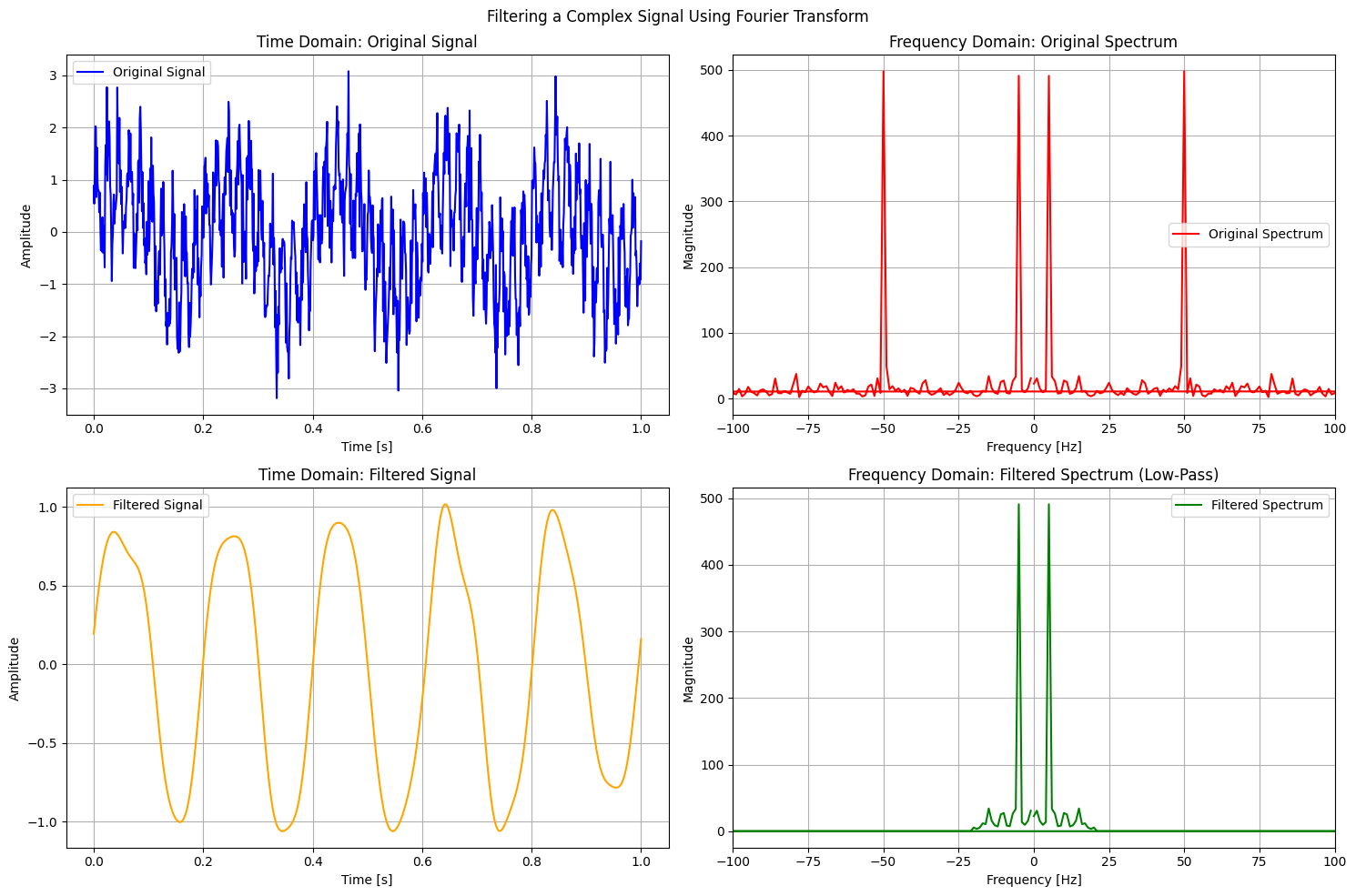
In this example, we start with a complex signal composed of multiple sinusoidal components and random noise. We apply a low-pass filter in the frequency domain to attenuate high-frequency components, resulting in a smoother signal in the time domain.
1. Initial Signal#
The original signal is a combination of:
A low-frequency sine wave component
A high-frequency sine wave component
Additive random noise
2. Fourier Transform#
We compute the Fourier Transform of the signal to obtain its frequency representation. This allows us to identify which frequencies dominate the signal and decide which ones to modify.
3. Applying the Low-Pass Filter#
A low-pass filter allows low frequencies to pass while attenuating high frequencies. We create a filter in the frequency domain that multiplies the Fourier coefficients, reducing the amplitude of frequencies beyond a certain cutoff.
4. Inverse Fourier Transform#
We then compute the Inverse Fourier Transform of the filtered frequency representation to obtain the modified signal in the time domain, demonstrating the effect of the filtering operation.
Visualization#
The following plots show:
Original Signal in the time domain.
Frequency Spectrum of the original signal.
Filtered Frequency Spectrum after applying the low-pass filter.
Filtered Signal in the time domain.
import numpy as np
import matplotlib.pyplot as plt

# Step 1: Generate a complex signal with multiple frequency components
np.random.seed(0)  # For reproducibility
t = np.linspace(0, 1, 1000)
low_freq = np.sin(2 * np.pi * 5 * t)  # Low frequency component (5 Hz)
high_freq = np.sin(2 * np.pi * 50 * t)  # High frequency component (50 Hz)
noise = 0.5 * np.random.randn(len(t))  # Random noise
signal = low_freq + high_freq + noise  # Combined signal

# Step 2: Compute the Fourier Transform of the signal
signal_fft = np.fft.fft(signal)
frequencies = np.fft.fftfreq(len(t), d=t[1] - t[0])

# Step 3: Create a low-pass filter (cutoff frequency = 20 Hz)
cutoff = 20  # Define cutoff frequency
filter_mask = np.abs(frequencies) <= cutoff  # Filter mask

# Step 4: Apply the filter to the Fourier coefficients
filtered_fft = signal_fft * filter_mask

# Step 5: Inverse Fourier Transform to get the filtered signal
filtered_signal = np.fft.ifft(filtered_fft)

# Plotting the results
fig, ax = plt.subplots(2, 2, figsize=(15, 10))

# Original signal in the time domain
ax[0, 0].plot(t, signal, color='b', label='Original Signal')
ax[0, 0].set_title('Time Domain: Original Signal')
ax[0, 0].set_xlabel('Time [s]')
ax[0, 0].set_ylabel('Amplitude')
ax[0, 0].legend()
ax[0, 0].grid()

# Frequency domain: Original signal
ax[0, 1].plot(frequencies, np.abs(signal_fft), color='r', label='Original Spectrum')
ax[0, 1].set_title('Frequency Domain: Original Spectrum')
ax[0, 1].set_xlabel('Frequency [Hz]')
ax[0, 1].set_ylabel('Magnitude')
ax[0, 1].set_xlim(-100, 100)
ax[0, 1].legend()
ax[0, 1].grid()

# Frequency domain: Filtered signal
ax[1, 1].plot(frequencies, np.abs(filtered_fft), color='g', label='Filtered Spectrum')
ax[1, 1].set_title('Frequency Domain: Filtered Spectrum (Low-Pass)')
ax[1, 1].set_xlabel('Frequency [Hz]')
ax[1, 1].set_ylabel('Magnitude')
ax[1, 1].set_xlim(-100, 100)
ax[1, 1].legend()
ax[1, 1].grid()

# Filtered signal in the time domain
ax[1, 0].plot(t, filtered_signal.real, color='orange', label='Filtered Signal')
ax[1, 0].set_title('Time Domain: Filtered Signal')
ax[1, 0].set_xlabel('Time [s]')
ax[1, 0].set_ylabel('Amplitude')
ax[1, 0].legend()
ax[1, 0].grid()

# Show the plots
plt.suptitle('Filtering a Complex Signal Using Fourier Transform')
plt.tight_layout()
plt.show()

